Code Download Address

Paper Record

计数的基本方法是确定边的数量,通过子图完全图边和点的关系来计算点数,最后得到答案
top n bounding box

首先处理出处理出top n的注意力权重和对应的bounding box

1
2
3
4
5
6
def filter_most_important(self, n, boxes, attention):
""" Only keep top-n object proposals, scored by attention weight """
attention, idx = attention.topk(n, dim=1, sorted=False)
idx = idx.unsqueeze(dim=1).expand(boxes.size(0), boxes.size(1), idx.size(1))
boxes = boxes.gather(2, idx)
return boxes, attention

boxes的shape为(n, 4, m),attention的shape为(n, m),其中n为batch size,m为一张图中bbox的数量

1
torch.topk(input, k, dim=None, largest=True, sorted=True, out=None) → (Tensor, LongTensor)

k表示top k,dim为指定维度,如果未指定则默认最后一维,largest表示返回最大还是最小(True/False),sorted表示返回的top k是否需要排序,out可选输出张量(Tensor, LongTensor)

返回值是一个元组(values,indices)

源码中指定的dim=1是bbox维度,即选取attention权值最大的k个bbox

1
torch.unsqueeze(input, dim) → Tensor

unsqueeze用于维度扩充,dim为插入的维度下标

expand是将torch的各个维度扩展到更大的尺寸,在unsqueeze之后,idx变为(n,1,m),然后扩展为(n,4,m),和bbox的tensor尺寸相同

1
torch.gather(input, dim, index, out=None, sparse_grad=False) → Tensor

gather函数在dim维度按照index对input进行索引把对应的数据提取出来的,这里是提取出top k的attention权值对应的bbox

Calculate A && D

然后计算注意矩阵和距离矩阵

1
2
relevancy = self.outer_product(attention)
distance = 1 - self.iou(boxes, boxes)

看下矩阵外积(outer_produce)的实现

1
2
3
4
5
6
7
8
9
10
def outer(self, x):
size = tuple(x.size()) + (x.size()[-1],)
a = x.unsqueeze(dim=-1).expand(*size)
b = x.unsqueeze(dim=-2).expand(*size)
return a, b

def outer_product(self, x):
# Y_ij = x_i * x_j
a, b = self.outer(x)
return a * b

(x.size()[-1],)表示将x.size()的最后一维取出并将其表示为元组,元组相加是拼接而非按位相加,得到size为(n,m,m),所以outer的作用就是将x变成两个(n,m,m)的tensor,将权值放在对应的倒数第一维和倒数第二维,outer_product将x转化后得到的a和b相乘得到外积

看一下Intersection over Union(IoU)的实现

1
2
3
4
5
6
def iou(self, a, b):
# this is just the usual way to IoU from bounding boxes
inter = self.intersection(a, b)
area_a = self.area(a).unsqueeze(2).expand_as(inter)
area_b = self.area(b).unsqueeze(1).expand_as(inter)
return inter / (area_a + area_b - inter + 1e-12)

先看一下 intersection

1
2
3
4
5
6
7
8
9
10
11
12
13
def intersection(self, a, b):
size = (a.size(0), 2, a.size(2), b.size(2))
min_point = torch.max(
a[:, :2, :].unsqueeze(dim=3).expand(*size),
b[:, :2, :].unsqueeze(dim=2).expand(*size),
)
max_point = torch.min(
a[:, 2:, :].unsqueeze(dim=3).expand(*size),
b[:, 2:, :].unsqueeze(dim=2).expand(*size),
)
inter = (max_point - min_point).clamp(min=0)
area = inter[:, 0, :, :] * inter[:, 1, :, :]
return area

a[:, :2, :]表示将dim=1的前两个切片(左上角坐标)取出,对应的a[:, 2:, :]则为右下角坐标

1
torch.max(input, other, out=None) → Tensor

torch.max可以将取两个tensor对应位置的最大值,返回是一个tensor,两个tensor不一样大时可以广播计算,不过这里源码直接将其拉伸成一样大的了

将左上角取最大值就得到了相交区域的上界,同理,右下角取最小值得到了相交区域的下界

1
torch.clamp(input, min, max, out=None) → Tensor

clamp给tensor的元素限定上下界(min,max),如果两个bbox没有交集,则可能计算出来的是负数,所以需要设定下界0,将两个inter对应的长宽相乘得到每两个bbox的相交面积area,得到面积交矩阵

然后看一下area

1
2
3
4
def area(self, box):
x = (box[:, 2, :] - box[:, 0, :]).clamp(min=0)
y = (box[:, 3, :] - box[:, 1, :]).clamp(min=0)
return x * y

显然计算的是bbox的面积,同时用了clamp做了极小限制防止出现负数

在iou中将得到的area通过unsqueeze在矩阵上横向扩展和纵向扩展,相加再减去面积交矩阵即可得到面积并矩阵,IoU = 面积交/面积并,计算即可

然后用得到的注意力矩阵A和距离矩阵D去计算$\bar{A}$

intra-object dedup

1
score = self.f[0](relevancy) * self.f[1](distance)

将A和D通过两个不同的激活函数,然后点乘来消除intra-object

来看一下激活函数的实现

在__init__里有

1
self.f = nn.ModuleList([PiecewiseLin(16) for _ in range(16)])

查看作者写的分段线性函数PiecewiseLin

1
2
3
4
5
6
7
8
9
10
11
12
13
14
15
16
17
18
19
20
21
22
23
24
25
26
27
28
29
class PiecewiseLin(nn.Module):
def __init__(self, n):
super().__init__()
self.n = n
self.weight = nn.Parameter(torch.ones(n + 1))
# the first weight here is always 0 with a 0 gradient
self.weight.data[0] = 0

def forward(self, x):
# all weights are positive -> function is monotonically increasing
w = self.weight.abs()
# make weights sum to one -> f(1) = 1
w = w / w.sum()
w = w.view([self.n + 1] + [1] * x.dim())
# keep cumulative sum for O(1) time complexity
csum = w.cumsum(dim=0)
csum = csum.expand((self.n + 1,) + tuple(x.size()))
w = w.expand_as(csum)

# figure out which part of the function the input lies on
y = self.n * x.unsqueeze(0)
idx = Variable(y.long().data)
f = y.frac()

# contribution of the linear parts left of the input
x = csum.gather(0, idx.clamp(max=self.n))
# contribution within the linear segment the input falls into
x = x + f * w.gather(0, (idx + 1).clamp(max=self.n))
return x.squeeze(0)

cumsum是累加

1
torch.cumsum(input, dim, out=None, dtype=None) → Tensor

返回的tensor y满足$y_i=x_1+x_2+\dots+x_i$

通过w=w/w.sum()和self.weight.data[0] = 0保证$f_k(0)=0,f_k(1)=1$

inter-object dedup

然后消除inter-object,方法是等比例缩小边的权重

1
2
3
dedup_score = self.f[3](relevancy) * self.f[4](distance)
dedup_per_entry, dedup_per_row = self.deduplicate(dedup_score, attention)
score = score / dedup_per_entry

dedup_score就是计算了式中的X,$X = f_4(A)\odot f_5(D)$

看一下deduplicate函数

1
2
3
4
5
6
7
8
9
10
def deduplicate(self, dedup_score, att):
# using outer-diffs
att_diff = self.outer_diff(att)
score_diff = self.outer_diff(dedup_score)
sim = self.f[2](1 - score_diff).prod(dim=1) * self.f[2](1 - att_diff)
# similarity for each row
row_sims = sim.sum(dim=2)
# similarity for each entry
all_sims = self.outer_product(row_sims)
return all_sims, row_sims

其中用了一个outer_diff函数

1
2
3
4
5
def outer_diff(self, x):
# like outer products, except taking the absolute difference instead
# Y_ij = | x_i - x_j |
a, b = self.outer(x)
return (a - b).abs()

和outer_product的功能类似,用这个函数求了attention的两两权重差和dedup_score的两两差,按照式子计算了proposal两两之间的相似度

1
torch.prod(input, dim, keepdim=False, dtype=None) → Tensor

prod是对指定维度dim求元素积,对应公式中的$\prod$

$row_sims$计算了proposal i和其它proposal相似的次数

对于$edge_{ij}$来说值需要除以${row_sims}_i$和${row_sims}_j$,所以这里处理了$row_sims$的$outer_product$,即$all_sims$

然后对score进行了缩放,即得到了$\bar{A}\odot ss^T$

aggregate the score

答案统计用的是$|V|=\sqrt{|E|}$,因此还需要将在intra-object dedup中消去的自环加回来

1
2
3
4
correction = self.f[0](attention * attention) / dedup_per_row
score = score.sum(dim=2).sum(dim=1, keepdim=True) + correction.sum(dim=1, keepdim=True)
score = (score + 1e-20).sqrt()
one_hot = self.to_one_hot(score)

算自环直接attention点积然后除倍率,矩阵点积对于边权值是线性变化,所以乘s而不是乘$s\odot s$,原式中diag是将数值填入对角矩阵的对角线,因为代码中是直接计数所以不需要这步操作

直接求和得到了|E|,开方即可得到|V|,也就是正确的计数

并将答案转化为特殊的one-hot编码$o=[o_0,o_1,\dots,o_n]^T$

$o_i=max(0,1-|c-i|)$

若答案为整数,则one-hot编码结果为对应答案位置为1,其余位置为0,否则o对应两个one-hot编码的线性插值

1
2
3
4
5
6
7
8
9
10
11
12
13
14
15
16
17
18
def to_one_hot(self, scores):
""" Turn a bunch of non-negative scalar values into a one-hot encoding.
E.g. with self.objects = 3, 0 -> [1 0 0 0], 2.75 -> [0 0 0.25 0.75].
"""
# sanity check, I don't think this ever does anything (it certainly shouldn't)
scores = scores.clamp(min=0, max=self.objects)
# compute only on the support
i = scores.long().data
f = scores.frac()
# target_l is the one-hot if the score is rounded down
# target_r is the one-hot if the score is rounded up
target_l = scores.data.new(i.size(0), self.objects + 1).fill_(0)
target_r = scores.data.new(i.size(0), self.objects + 1).fill_(0)

target_l.scatter_(dim=1, index=i.clamp(max=self.objects), value=1)
target_r.scatter_(dim=1, index=(i + 1).clamp(max=self.objects), value=1)
# interpolate between these with the fractional part of the score
return (1 - f) * Variable(target_l) + f * Variable(target_r)

最后考虑尽可能用A和D矩阵中为1和0的数字来计算答案,计算两个置信系数,然后返回最终的计数特征

1
2
3
4
5
one_hot = self.to_one_hot(score)
att_conf = (self.f[5](attention) - 0.5).abs()
dist_conf = (self.f[6](distance) - 0.5).abs()
conf = self.f[7](att_conf.mean(dim=1, keepdim=True) + dist_conf.mean(dim=2).mean(dim=1, keepdim=True))
return one_hot * conf